An Exploration of the Relationship Between Measures of Compactness and Transport Choices

An 1,310-word essay for ENVS469 Trends Outcomes Impacts. Using two sets of analyses conducted with SPSS, the essay examines whether more compact communities in North West England have lower car ownership and higher public transportation usage. The essay earned a 72, a distinction. Written in November 2016.

1. Introduction

Climate change has increased the focus on sustainable transport. Personal motor vehicles emit most transportation-related greenhouse gases (Union of Concerned Scientists) and researchers (Erickson and Tempest 2014) argue cities are essential to promote sustainable public transport systems. This paper investigates whether compact cities lead to more sustainable transport. Two types of statistical analyses were conducted using a sample of 2011 Census data from England’s Northwest region.

 2. Spatial Setting and Transport Mode

The first set of analyses examines the categorised share (i.e., low, medium, high) of car or van ownership (i.e., zero, one, or two or more) compared to spatial setting (i.e., metropolitan and non-metropolitan). A fourth analysis looks at the categorised share of commuters using public transport. Census data at the Local Authority District level was used. Table 2.1 has descriptive statistics for the first three analyses.

Table 2.1: Descriptive Statistics for Car and Van Ownership in Local Authorities in the Northwest of England (2011)

		Households Without a Car or Van (%)	Households with One Car or Van (%)	Households with 2+ Cars or Vans (%)
N	Valid	39	39	39
	Missing	0	0	0
Mean		25.8000	43.0640	31.1360
Median		24.6825	43.1460	30.2656
Std. Deviation		7.81859	1.69917	7.53208
Range		33.13	8.86	30.92
Minimum		13.00	38.14	14.85
Maximum		46.14	47.01	45.77

For categorisation, values within one standard deviation from the mean are medium, which is appropriate because mean and average are synonyms for medium. Values greater than one standard deviation are too far above or below average to be medium, so they are high or low, respectively.

For households without a vehicle, low is less than 18%, medium is 18—33.6%, and high is greater than 33.6%. Table 2.2 is a crosstabulation table, while Table 2.3 indicates the Chi-Square value.

Table 2.2: Crosstabulation of Households without a Car or Van by Metropolitan Area in the Northwest of England (2011)

		Metropolitan	Non-Metropolitan	Total
Households without a car or van	Low	0	6	6
	Medium	11	17	28
	High	4	1	5
Total		15	24	39

Table 2.3: Chi-Square Test of Households without a Car or Van by Metropolitan Area in the Northwest of England (2011)

	Value	df	Asymptotic Significance (2-sided)
Pearson Chi-Square	7.403a	2	.025
Likelihood Ratio	9.445	2	.009
Linear-by-Linear Association	7.212	1	.007
N of Valid Cases	39
a. 4 cells (66.7%) have expected count less than 5. The minimum expected count is 1.92.

All metropolitan areas are medium to high and all non-metropolitan areas are low to medium (except Blackpool). These results suggest not owning a vehicle may be related to spatial setting. However, most local authorities are medium, so a definitive conclusion is not possible. The Chi-Square value, 0.025, indicates a low probability that the result is due to random chance.

The next analysis looked at households with one vehicle. The standard deviation (Table 2.1) is only about 1.7, indicating the dataset is tightly distributed around the mean. Consequently, it is not appropriate to define categories for this analysis, and a relationship between the two variables is unlikely to be statistically significant.

The third analysis is households with two or more vehicles. Using standard deviation (Table 2.1), the categories are: low is less than 23.6%, medium is 23.6%—38.7%, and high is greater than 38.7%. Table 2.4 is a crosstabulation table, while Table 2.5 shows the Chi-Square significance value.

Table 2.4: Crosstabulation of Households with Two or More Cars or Vans by Metropolitan Area in the Northwest of England (2011)

		Metropolitan	Non-Metropolitan	Total
Households with Two or More Cars or Vans	Low	4	2	6
	Medium	11	13	24
	High	0	9	9
Total		15	24	39

Table 2.5: Chi-Square Test of Households with Two or More Cars or Vans by Metropolitan Area in the Northwest of England (2011)

	Value	df	Asymptotic Significance (2-sided)
Pearson Chi-Square	8.193a	2	.017
Likelihood Ratio	11.227	2	.004
Linear-by-Linear Association	7.404	1	.007
N of Valid Cases	39
a. 3 cells (50.0%) have expected count less than 5. The minimum expected count is 2.31.

Metropolitan areas are low to medium. All but two non-metropolitan areas (Blackpool and Barrow-in-Furness) are medium to high. The analysis suggests that ownership of two or more vehicles may be related to spatial setting, but most local authorities are again medium. This result is unlikely to be due to random chance (Chi-Square is 0.017).

The fourth analysis investigated public transport use by commuters. Table 2.6 shows the descriptive statistics.

Table 2.6: Descriptive Statistics for Commuter Use of Public Transport in Local Authorities in the Northwest of England (2011)

N	Valid	39
	Missing	0
Mean		10.0610
Median		8.3135
Std. Deviation		5.43118
Range		23.96
Minimum		3.45
Maximum		27.40

Using standard deviation, the categories are: low is less than 4.6% of commuters using public transport, medium is 4.6%—15.5%, and high is greater than 15.5%. Table 2.7 is a crosstabulation table, while Table 2.8 indicates the Chi-Square significance value.

Table 2.7: Crosstabulation of Commuters Taking Public Transport by Metropolitan Area in the Northwest of England (2011)

		Metropolitan	Non-Metropolitan	Total
Commuters Taking Public Transport	Low	0	3	3
	Medium	11	21	32
	High	4	0	4
Total		15	24	39

Table 2.8: Chi-Square Test of Commuters Taking Public Transport by Metropolitan Area in the Northwest of England (2011)

	Value	df	Asymptotic Significance (2-sided)
Pearson Chi-Square	8.501a	2	.014
Likelihood Ratio	10.786	2	.005
Linear-by-Linear Association	7.715	1	.005
N of Valid Cases	39
a. 4 cells (66.7%) have expected count less than 5. The minimum expected count is 1.15.

The crosstabulation shows that metropolitan areas are medium to high compared to low to medium in non-metropolitan areas, suggesting a relationship between public transport use and spatial setting. However, most local authorities are again medium. This relationship is unlikely to be due to random chance (Chi-Square is 0.014).

3. Population Density and Transport Mode

The next set of analyses accounts for the variability of densities within local authorities by looking at the relationship between population density and transport choices at the Middle-Layer Super-Output Area (MSOA) level. For each analysis, a scatterplot was prepared and the correlation coefficient (Pearson’s r) and coefficient of determination (R²) was calculated.

The first three analyses (Graphs 3.1-3.3 and Tables 3.1-3.3) look at the percentage of households with cars or vans (i.e., zero, one, two or more) compared to population density. Graph 3.1 and Table 3.1 are for households without a vehicle.

Graph 3.1: Relationship between Population Density and the Percentage of Households without Cars or Vans in the Northwest of England (2011)

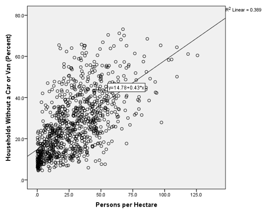
The above scatterplot and line of best fit indicate that a positive relationship exists between the two variables.

Table 3.1: Correlation between Population Density and the Percentage of Households without Cars or Vans in the Northwest of England (2011)

		Persons per Hectare	Households without a Car or Van (%)
Persons per Hectare	Pearson Correlation	1	.624**
	Sig. (2-tailed)		.000
	N	924	924
Households without a Car or Van (%)	Pearson Correlation	.624**	1
	Sig. (2-tailed)	.000
	N	924	924
**. Correlation is significant at the 0.01 level (2-tailed).

The r value, 0.624, confirms the interpretation of the scatterplot. The R² value means that 38.9% of the variation in households without vehicles is explained by population density (and vice versa). The result is unlikely to be due to random chance (i.e., significant at the 0.01 level).

The next analysis (Graph 3.2 and Table 3.2) examines households with one vehicle.

 Graph 3.2: Relationship between Population Density and the Percentage of Households with One Car or Van in the Northwest of England (2011)

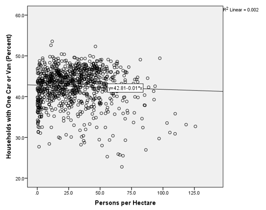
The relationship between vehicle ownership and population density is not obvious, but the line of best fit shows a weak negative relationship.

Table 3.2: Correlation between Population Density and the Percentage of Households without One Car or Van in the Northwest of England (2011)

		Persons per Hectare	Households with One Car or Van (%)
Persons per Hectare	Pearson Correlation	1	-.050
	Sig. (2-tailed)		.130
	N	924	924
Households with One Car or Van (%)	Pearson Correlation	-.050	1
	Sig. (2-tailed)	.130
	N	924	924

 The r value, -0.05, confirms the interpretation of the scatterplot. The R² value is only 0.2%, indicating limited predictive power. In addition, the result may be due to random chance (i.e., not statistically significant).

Graph 3.3 and Table 3.3 are for households with two or more vehicles.

Graph 3.3: Relationship between Population Density and the Percentage of Households with Two or More Cars or Vans in the Northwest of England (2011)

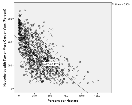
The scatterplot and line of best fit show a negative relationship between the two variables.

Table 3.3: Correlation between Population Density and the Percentage of Households without Two or More Cars or Vans in the Northwest of England (2011)

		Persons per Hectare	Households with 2+ Cars or Vans (%)
Persons per Hectare	Pearson Correlation	1	-.639**
	Sig. (2-tailed)		.000
	N	924	924
Households with 2+ Cars or Vans (%)	Pearson Correlation	-.639**	1
	Sig. (2-tailed)	.000
	N	924	924
**. Correlation is significant at the 0.01 level (2-tailed).

Pearson’s correlation coefficient, -0.639, indicates a strong negative relationship between the two variables, and the R² value demonstrates that 40.9% of the variation in multiple vehicle ownership is explained by density (and vice versa). The result is unlikely due to random chance (i.e., significant at 0.01 level).

The final analysis is the share of commuters using public transport versus density (Graph 3.4 and Table 3.4).

Graph 3.4: Relationship between Population Density and Commuters Using Public Transport in the Northwest of England (2011)

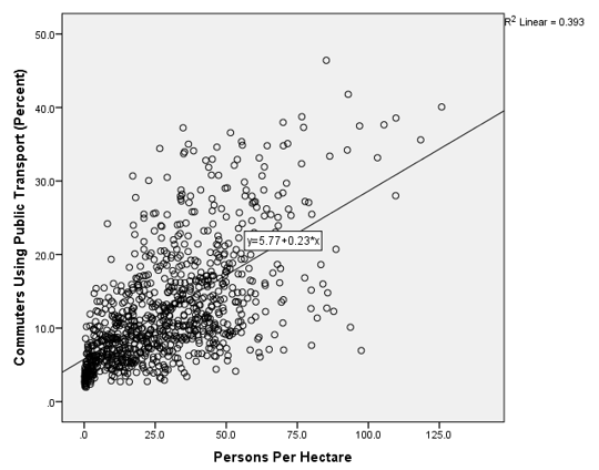
The scatterplot and line of best fit reveals a positive relationship between density and public transport use by commuters.

Table 3.4: Correlation between Population Density and the Percentage of Workers Commuting by Public Transit in the Northwest of England (2011)

		Workers Commuting by Public Transit (%)	Persons per Hectare
Workers Commuting by Public Transit (%)	Pearson Correlation	1	.627**
	Sig. (2-tailed)		.000
	N	924	924
Persons per Hectare	Pearson Correlation	.627**	1
	Sig. (2-tailed)	.000
	N	924	924
**. Correlation is significant at the 0.01 level (2-tailed).

Pearson’s correlation coefficient, 0.627, confirms the interpretation of the scatterplot. The R² value indicates that 39.3% of the variation in density explains the variation in commuters taking public transport (and vice versa). The result is unlikely due to random chance (i.e., significant at 0.01 level).

 4. Discussion of the Analytical Approaches

Both types of analyses help to assess whether compact cities lead to more sustainable transport, but they have important shortcomings.

The spatial setting analyses do not directly address compactness. For example, Blackpool is the third densest local authority in the dataset, but is non-metropolitan. Halton (non-metropolitan) is also denser than Oldham (metropolitan). Those nuances are lost in the crosstabulation, which does not consider population density. This lack of nuance may contribute to most local authorities being ‘medium’ in the private vehicle and public transport analyses. A density-based approach to categorising metropolitan/non-metropolitan areas may help mitigate this issue.

The second type of analysis is an improvement by specifically looking at population density, but the relatively small MSOA scale also has shortcomings. For example, Blackburn with Darwen 004 is the seventh densest MSOA, but is ranked 676 (out of 924) for commuters using public transport. This outcome may be because the entire Blackburn with Darwen local authority (classified as non-metropolitan) may be less dense than the individual MSOA and may not support a comprehensive public transport network. Unfortunately, by looking at a relatively small geographic area, the density of individual MSOAs does not mean that sufficient density exists in the surrounding area to discourage driving and promote public transport.

Analysing data for additional years, UK regions, and/or countries would bolster the conclusions of the each analysis by reducing the likelihood that the relationships are spurious. For example, in 2011 petrol averaged £134/L compared to £112/L in 2015 (Petrol Prices). The higher price of petrol in 2011 may have increased the percentage of commuters using public transport. Repeating the analysis for additional years would help determine whether the relationships with density/metropolitan areas persist despite fluctuations in petrol prices (and other factors). In addition, assessing data from other UK regions and/or countries would help to test whether the findings are unique to the Northwest of England or are applicable more broadly.

 5. Conclusion

The findings from these analyses help to demonstrate that more compact cities lead to greater percentages of people living without (or with fewer) private vehicles and more commuters using public transport. These findings are expected because higher densities make both public transit more viable, by having more potential riders, and commuting by private vehicles less desirable due to increasing congestion on roads. Additional research is essential to validate the tentative conclusions reached by these analyses.

 

6. Bibliography

Erickson, P. and Tempest, K. (2014). ‘Advancing climate ambition: How city-scale actions can contribute to global climate goals’, Stockholm Environment Institute, Working Paper No. 2014-06.

Petrol Prices (n.d.). The price of fuel. Available at: https://www.petrolprices.com/the-price-of-fuel.html (accessed 27 October 2016).

Union of Concerned Scientists (n.d.). Cars and global warming. Available at: http://www.ucsusa.org/clean-vehicles/car-emissions-and-global-warming#.WBCFYWgrKUk (accessed 26 October 2016).